You often see people post about the kelly criterion and how to use it to maximize your gains over time when investing. When they post these articles though they often cut and paste an equation for best bet size. The equation comes from the original paper by Kelly but what they don’t realize is that the optimal bet size is dependent on the distirbution of returns for the game or asset you’re investing in. Why is this important? Well, Kelly was considering a situaiton where you get a signal for a binary event and the signal isn’t always right. That means, he was looking at a binomial distribution. Stock returns, however, generally follow a continuous distribution approximating a log normal distribution.
Before we get into the actual solution for using Kelly in investing we should probably walk through how you get to the equation for an optimal bet size.
First, we assume that we have an investment portfolio of value V. In every period we can place a bet with some fraction of that portfolio. If the bet wins we increase our portfolio size and if we lose we decrease our portfolio size. We assume that the investor wants to maximize their gains over time. To start with we have a few parameters: V (the value of the portfolio), f (the fraction of our portfolio we bet), and s (the asset we’re buying). Then the value of the portfolio in time one will be equal to the value of the portfolio in time zero plus the gains or losses from your bet. We can turn this into an equation as follows:

We can simplify the right hand side of the equation with a little bit of factoring:

Now we take the natural log of both sides and divide through by the value of the portfolio in the current time period which gives us the gain, G:

When people talk about solving for Kelly they mean that they want to solve for the optimal fraction f for long term gain G. The standard way to do this would be to take the derivative of the function with respect to f and then solve for f*. But the integral on the right is often unsolvable analytically for the types of distributions most investment assets follow meaning you need to resort to numerical methods.
One of the problems you’ll find trying to solve this integral if s has normally distributed returns is that you need to bound your possible returns to the upside and downside. You can see why when you consider the integral above. If the fraction you bet times the return s is ever less than 1 the logarithm in the integral will be undefined. This means that in reality, for most real asset return distributions, you will need to bound the possible returns. This could be achieved in practice through the use of stop losses or options strategies.
Let’s look at an example. Imagine we have an asset that historically returns 0.1% a month with a standard deviation of 6%. How much should you allocate to that asset every month to maximize the geometric growth of your portfolio?
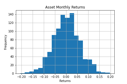
First, we can simulate the returns over time using python. When we do that 1000 times we get a distribution that looks like the following:

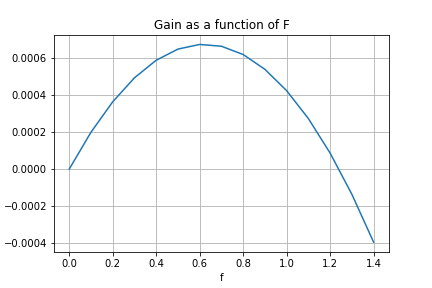
Next, we calculate the gain G for every value of f between 0 and 1.5. We also need to bound the returns on the lower end. Essentially we are modeling a stop loss where if we lose up to x on a stock we will sell it immediately. This is important because if we allow the term inside the integral to go negative we’ll get an undefined number (there is no log of a negative number). More practically, this means that if we use kelly we can never go broke, although we could still lose a lot of money.
When we plot this out we get the following curve:

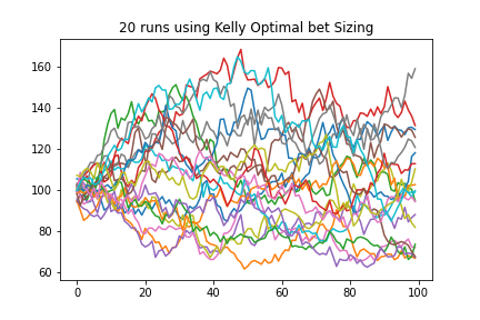
When we solve for the f that gives us the the maximum gain we get 0.6. That means that in this case we should bet 60 percent of our portfolio on every trade. What does this look like if we tried this 100 times? The chart below shows 20 simulated runs of this trading strategy over 100 trades while betting optimal kelly.

An important point to note here is that even betting kelly optimal you can still lose money in a positive expectancy trading strategy even over 100 bets. In fact, your results can vary wildly. This shows how difficult it is to know even after 100 bets if a trading strategy is long run profitable once you go live with it.