As a businesses grow they often try to find economies of scale in their processes. In this case we are defining a process as the steps needed to transform some set of inputs into a product, or output. As volumes grow there is an opportunity to improve your efficiency by splitting tasks between different groups and allowing specialization.
A simple example can illustrate this effort. Imagine you are an entrepreneur manufacturing a product. Your first prototype is probably built from start to finish by one person, perhaps in your garage. As time goes on and your product gains traction in the market you could begin to split up the tasks into an assembly line, allowing for more efficiency as total production volumes increase.
Once you decide to split up the processes involved in producing an item you often then look to design sub processes that are “efficient”. What do we mean by efficient? Let’s start by considering a simple model of what the business is trying to do. We can say that the business is trying to maximize their profits, and that profits are equal to sales revenue minus the cost of making the product. When designing a process we can’t impact sales (at least not directly) but we can impact the cost of producing the good. Because of this, most process design is an exercise in minimizing cost. We say that a process that costs less than another process is more efficient.
Practically how does this play out? Often a team will build an excel model of different options for how to complete a process. They’ll then estimate the average value of some inputs and plug them into their model. Whichever process has the lowest average cost is generally selected. Then the team implements the process and often finds that the realized cost after implementation is higher than what they estimated. Why does this happen and is there a better approach?
Various process improvement methods, like Lean and Six Sigma, propose that variation is what causes the difference between expected process performance and actual process performance. Most of the time they never actually say why that is the case though. They treat that idea as almost axiomatic. However, there is a simple explanation for the impact of variation on process results. In general, the delta in expected versus actual process performance is due to ignoring the impact of variation on process design. I’ll propose a different approach to process improvement and show how incorporating an understanding of variation of inputs into process design can lead to better results.
The first step when comparing different options for process is to develop a cost function for each potential sequence of steps that will be taken by a person. This cost function should incorporate the key variables that will impact cost, and ignore any minor details. For example, say there are 3 variables that impact the cost of a process: x, y and z. If the majority of the cost is driven by variable x, you’re generally better off focusing on that variable. A model is supposed to be a simplified version of the real world. In this case let’s imagine that variable x is the key factor impacting process costs. We develop two processes and estimate a cost function for each process. We model the cost as a function of a parameter x.
The first process has the following cost function:

And the second process has the following cost function:

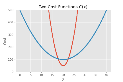
We can graph both functions in the coordinate plane where the vertical axis is cost and the horizontal axis is the input x.

If we backtrack for a minute to the excel scenario we can make a few observations. If the average x is 20 and we put that number in our spreadsheet we will select the process outlined in red (process 1) as the most efficient process. Is it though? The key insight here is that x is generally a random variable. Because of that the actual average cost will be dependent on the variation we see in x.

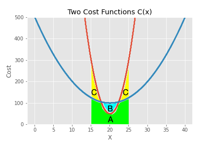
A simple integration could give us the average cost of processing a good based on a range of values of x. For example, if x uniformly varies from 15 to 25 than the average cost for process 1 will be the area A plus C. The average cost for process 2 will be the area of A plus B. While an integration would get us the answer for average cost it can sometimes be more intuitive to simulate X and look at the results.
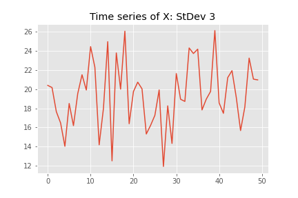
In the following chart we show a time series of simulated X variables. We assume that on average X is 20, X is normally distributed, and has a standard deviation of 3.

If we calculate the average cost of our process based on this random variable X we get 163.9 for process 1 (reminder: in red above). However, if we run the same cost analysis on the second process we get an average cost of 111.4. How does this happen? Once the variation is taken into account the second process (in blue) actually has a lower average cost. The variation in the input x is very important. In this case the average cost is impacted by the times that x drifts to away from the optimal value at 20.
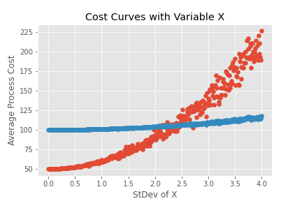
What if we run this analysis for multiple types of X, starting with a standard deviation of 0 and working our way up? If we plot both average costs we may find something interesting.

Again, process 1 is in red and the curve shows the average processing cost at different levels of variation for the random variable of x. We find that as long as the variation of the x is below 2.5 the average cost for process 1 is less than the average cost for process 2. Once the standard deviation in x rises above 2.5 we would be better using process 2 even though the cost of process 2 at an average value of X is higher than the cost of process 1 at the average X. To put this another way, the cost of a process at the average of an input value does not equal the average cost of the process! This is really important!
Another key point is that the cost of both processes increases as the variation in x increases. In both cases x always has an average value of 20. The only thing that changes is the standard deviation of x. As the variation in x increases the cost of both processes also increases. However, process two, which has a much flatter cost curve than process one, increases cost at a lower rate. We call this “flatness” in the curve “process flexibility”.
There are a few key takeaways from this simple example. First, we have to understand the cost curve of a potential process, not just the cost at the average value of an input. Second, the reason process improvement focuses on reducing variation is that reducing variation really does lead to lower average costs! Third, the flatter our cost curve the more flexible the process is and that flexibility leads to real impacts on average cost. And remember, to maximize profits we have to minimize cost!